Exploring probability distributions for bivariate temporal granularities
Sayani Gupta
Sayani07
@SayaniGupta07
https://sayanigupta-iisa2019.netlify.com/
International Indian Statistical Association
December 26, 2019
Electricity smart meter technology (~ 40 billion half hourly observations)
- Source : Department of the Environment and Energy, Australia
- Frequency: Half hourly (interval meter reading (Kwh))
- Time Span: 2012 to 2014
- Spread: 14K (approx.) households based in Newcastle, New South Wales, and parts of Sydney
Smart meters record electricity usage (per kWh) every 30 minutes and send this information to the electricity retailer for billing
Consumers can save considerable amount on their electricity bill by
- Switching on their hot water heater or do laundry when energy is cheaper, or when their solar system is generating surplus energy
- Switching off appliances during peak demands
- Check usage and compare with similar homes
Retailers can reduce costs and increase efficiency
- Lowering metering and connection fees
- Drawing insights into when customer is home, or sleeping, or even what appliances they are using based on usage figures
- Rewarding customers for mindful usage
Just to give you some perspective I have this data from Department of Energy and Environment, Australia that provides interval meter reading data every 30 minutes from 2012 to 2014. So you can think of it like, that the finest temporal unit here is half hour, whereas the coarsest temporal unit is year. This data is made available for 14k customers located in different local government areas across places.. So this is a data which is spread across both time and space and hence is a spatio-temporal data.
Visualize the raw data from from 2012 - 2014 for 50 households
Visualize the periodicities in half-hourly energy usage for 1 household from 2012 to 2014

Explorartory Data Analysis
"Same Stats, Different Graphs: Generating Datasets with Varied Appearance and Identical Statistics through Simulated Annealing"
Well, there can be numerous ways to analyse this data! But I was interested in answering the question - that given this huge volume and spread, how can one explore this data systematically?
Problem : How do we systematically explore large quantities of temporal data across different deconstructions of time (half-hour, day, type of day, year) to find regular patterns or anomalies in behaviour?
Solution : Visualize probability distributions over different time granularities.
Developed by John Tukey as a way of systematically using the tools of statistics on a problem before a hypotheses about the data were developed. This encourages to break the big problem into pieces and focusing on subsets. So the reduced goal that I set for myself is to look at time only and to provide ... . The smart meter example is the one that motivated me for this problem, how the idea is to provide the same for any temporal data following an hierarchy.
The key terms are decontructing time and visualizing distribution. In the next couples of slides, we will talk about the strength and challenges for each of these.
Visualize probability distributions over different time granularities
Time granularities
abstractions of time based on calendar
Arrangement
Linear
- days, weeks, months, years
Cyclic
- Circular day-of-week, month-of-year or hour-of-day
- Quasi-circular day-of-month, week-of-month
- Aperiodic public holidays, school vacations
Order
- Single-order-up second-of-minute, hour-of-day
- Multiple-order-up second-of-hour, hour-of-week
Data Structure for exploration
Extension of a tsibble - data abstraction for tidy temporal data
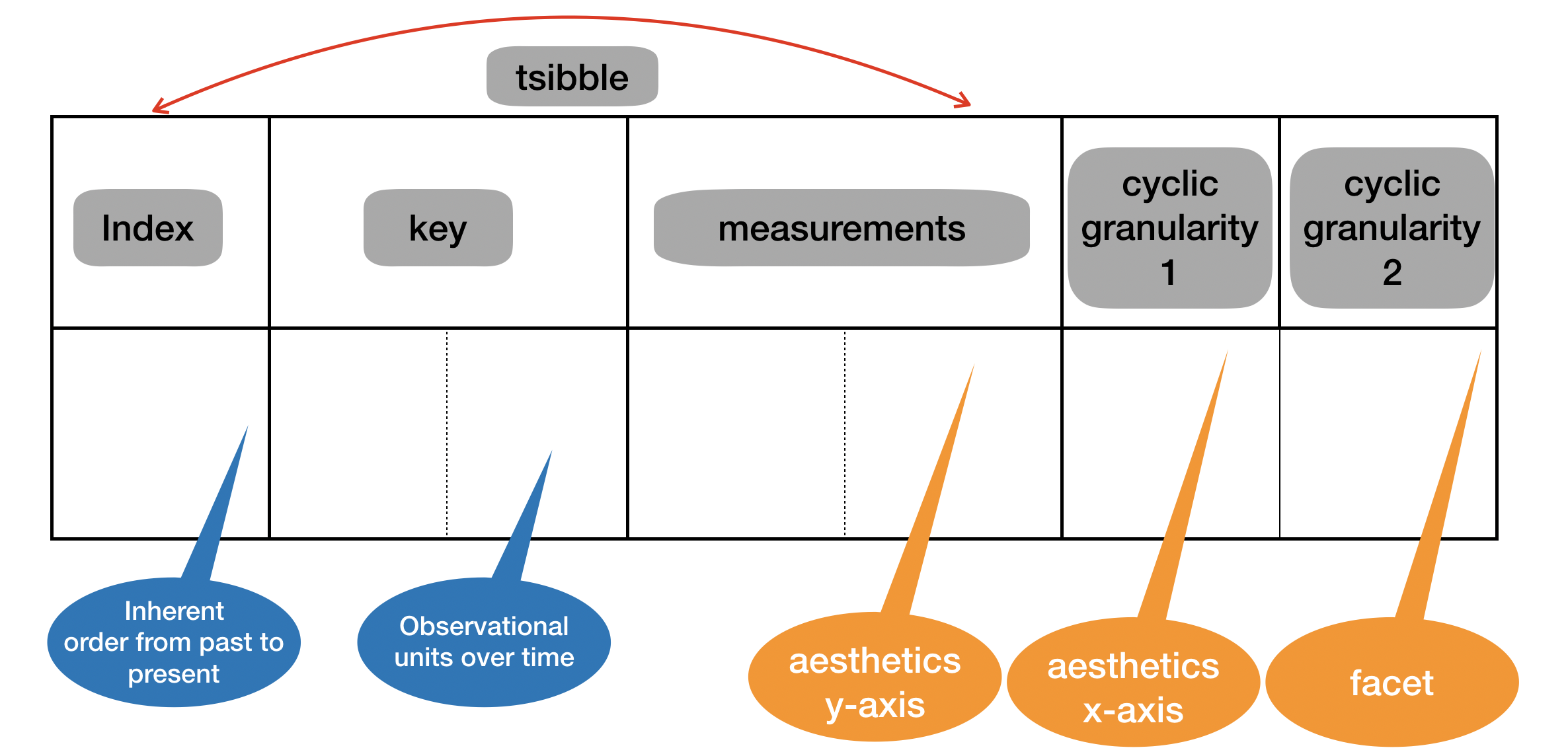
Relationship of cyclic granularities
Harmonies : pairs of granularities that aid exploratory data analysis
Clashes : pairs leading to structurally empty sets
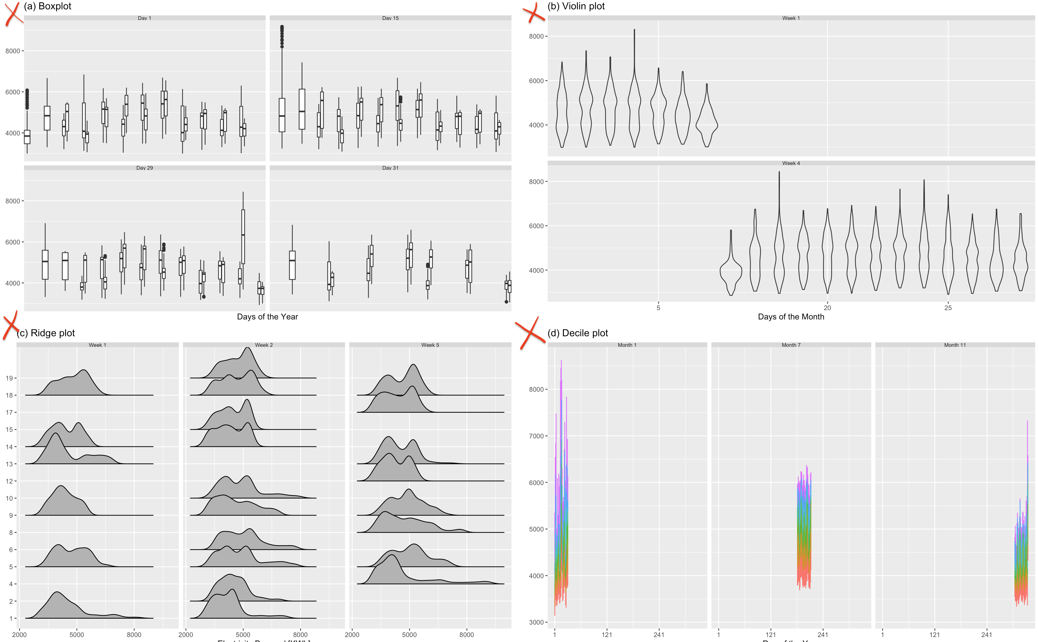
Summarising probability distributions
Types of statistical distribution plots

R package: gravitas
Computation
Compute any cyclic granularity? create_gran()
Exhaustive list of granularities to explore? search_gran()
Interaction
Check if cyclic granularities are harmonies/clashes? is.harmony()
List of harmonies to explore? harmony()
Visualization
Possible probability distributions plots for harmonies? prob_plot()
Sufficient observations? gran_obs()
Recommendation on a harmony? gran_advice()
smart meter example
- the data
#> # A tsibble: 1,450,232 x 8 [30m] <UTC>#> # Key: customer_id [50]#> customer_id reading_datetime general_supply_…#> <chr> <dttm> <dbl>#> 1 10006414 2012-02-10 08:00:00 0.141#> 2 10006414 2012-02-10 08:30:00 0.088#> 3 10006414 2012-02-10 09:00:00 0.078#> 4 10006414 2012-02-10 09:30:00 0.151#> # … with 1.45e+06 more rows, and 5 more variables:#> # event_key <dbl>, controlled_load_kwh <dbl>,#> # gross_generation_kwh <dbl>,#> # net_generation_kwh <dbl>, other_kwh <dbl>Data source : Department of the Environment and Energy, Australia
smart meter example
- the data
- possible cyclic granularities search_gran()
smart_meter %>% search_gran(lowest_unit = "hhour", highest_unit = "month", filter_out = c("fortnight", "hhour"))| x | |
|---|---|
| 1 | hour_day |
| 2 | hour_week |
| 3 | hour_month |
| 4 | day_week |
| 5 | day_month |
| 6 | week_month |
smart meter example
- the data
- possible cyclic granularities search_gran()
- set of harmonies harmony()
smart_meter %>% harmony(ugran = "month", lgran = "hhour", filter_out = c("fortnight", "hhour"))| facet_variable | x_variable | facet_levels | x_levels | |
|---|---|---|---|---|
| 1 | day_week | hour_day | 7 | 24 |
| 2 | day_month | hour_day | 31 | 24 |
| 3 | week_month | hour_day | 5 | 24 |
| 4 | day_month | hour_week | 31 | 168 |
| 5 | week_month | hour_week | 5 | 168 |
| 6 | day_week | hour_month | 7 | 744 |
| 7 | hour_day | day_week | 24 | 7 |
| 8 | day_month | day_week | 31 | 7 |
| 9 | week_month | day_week | 5 | 7 |
| 10 | hour_day | day_month | 24 | 31 |
| 11 | day_week | day_month | 7 | 31 |
| 12 | hour_day | week_month | 24 | 5 |
| 13 | day_week | week_month | 7 | 5 |
Good news! Only 13 out 30 are harmonies
smart meter example
- the data
- possible cyclic granularities search_gran()
- set of harmonies harmony()
- advice gran_advice()
smart_meter %>% gran_advice("month_year", "hour_day")#> The chosen granularities are harmonies #> #> Recommended plots are: quantile #> #> Number of observations are homogenous across facets #> #> Number of observations are homogenous within facets #> #> Cross tabulation of granularities : #> #> # A tibble: 24 x 13#> hour_day Jan Feb Mar Apr May Jun Jul#> <fct> <dbl> <dbl> <dbl> <dbl> <dbl> <dbl> <dbl>#> 1 0 1151 1095 730 660 682 1008 1054#> 2 1 1154 1094 730 660 682 1008 1054#> 3 2 1152 1094 730 660 682 1008 1054#> 4 3 1150 1094 730 660 682 1008 1054#> # … with 20 more rows, and 5 more variables:#> # Aug <dbl>, Sep <dbl>, Oct <dbl>, Nov <dbl>,#> # Dec <dbl> Quantile plots recommended for the harmony pair (month_year, hour_day)
smart meter example
- the data
- possible cyclic granularities search_gran()
- set of harmonies harmony()
- advice gran_advice()
- visualize harmonies prob_plot()
smart_meter %>% prob_plot("month_year","hour_day", plot_type = "quantile", response = "general_supply_kwh", quantile_prob = c(0.05, 0.1, 0.25, 0.5, 0.75, 0.9, 0.95)
Another example: Cricket data of Indian Premier League
Data source: Cricsheet , Kaggle
#> Observations: 136,598#> Variables: 38#> $ season <dbl> 2008, 2008, 2008, 2008, 200…#> $ match_id <dbl> 1, 1, 1, 1, 1, 1, 1, 1, 1, …#> $ inning <dbl> 1, 1, 1, 1, 1, 1, 1, 1, 1, …#> $ over <dbl> 1, 1, 1, 1, 1, 1, 1, 2, 2, …#> $ ball <dbl> 1, 2, 3, 4, 5, 6, 7, 1, 2, …#> $ winner <chr> "Kolkata Knight Riders", "K…#> $ total_runs <dbl> 1, 0, 1, 0, 0, 0, 1, 0, 4, …#> $ batting_team <chr> "Kolkata Knight Riders", "K…#> $ bowling_team <chr> "Royal Challengers Bangalor…#> $ batsman <chr> "SC Ganguly", "BB McCullum"…#> $ non_striker <chr> "BB McCullum", "SC Ganguly"…#> $ bowler <chr> "P Kumar", "P Kumar", "P Ku…#> $ is_super_over <dbl> 0, 0, 0, 0, 0, 0, 0, 0, 0, …#> $ wide_runs <dbl> 0, 0, 1, 0, 0, 0, 0, 0, 0, …#> $ bye_runs <dbl> 0, 0, 0, 0, 0, 0, 0, 0, 0, …#> $ legbye_runs <dbl> 1, 0, 0, 0, 0, 0, 1, 0, 0, …#> $ noball_runs <dbl> 0, 0, 0, 0, 0, 0, 0, 0, 0, …#> $ penalty_runs <dbl> 0, 0, 0, 0, 0, 0, 0, 0, 0, …#> $ batsman_runs <dbl> 0, 0, 0, 0, 0, 0, 0, 0, 4, …#> $ extra_runs <dbl> 1, 0, 1, 0, 0, 0, 1, 0, 0, …#> $ player_dismissed <chr> NA, NA, NA, NA, NA, NA, NA,…#> $ dismissal_kind <chr> NA, NA, NA, NA, NA, NA, NA,…#> $ fielder <chr> NA, NA, NA, NA, NA, NA, NA,…#> $ city <chr> "Bangalore", "Bangalore", "…#> $ date <date> 2008-04-18, 2008-04-18, 20…#> $ team1 <chr> "Kolkata Knight Riders", "K…#> $ team2 <chr> "Royal Challengers Bangalor…#> $ toss_winner <chr> "Royal Challengers Bangalor…#> $ toss_decision <chr> "field", "field", "field", …#> $ result <chr> "normal", "normal", "normal…#> $ dl_applied <dbl> 0, 0, 0, 0, 0, 0, 0, 0, 0, …#> $ win_by_runs <dbl> 140, 140, 140, 140, 140, 14…#> $ win_by_wickets <dbl> 0, 0, 0, 0, 0, 0, 0, 0, 0, …#> $ player_of_match <chr> "BB McCullum", "BB McCullum…#> $ venue <chr> "M Chinnaswamy Stadium", "M…#> $ umpire1 <chr> "Asad Rauf", "Asad Rauf", "…#> $ umpire2 <chr> "RE Koertzen", "RE Koertzen…#> $ umpire3 <lgl> NA, NA, NA, NA, NA, NA, NA,…Difference in strategy between two top teams
Special thanks to
 Di Cook
 NUMBATS, Monash University
 Rob J Hyndman
More Information
Package: gravitas 0.1.0 on CRAN
Slides: https://sayanigupta-iisa2019.netlify.com/
Materials: https://github.com/Sayani07/IISA2019
Slides created with Rmarkdown, knitr, xaringan, xaringanthemer